Earthquakes in the Greater San Francisco Bay Area
Back to Random Number Generators, Statistics, and ProbabilityThis is a report about the distribution of earthquakes for the year 1997 in the San Francisco Bay area with respect to magnitude, depth, and location. The specific area covered is enclosed by latitude 36.5 to 38.5 and longitude -121.0 to -123.5. You will see a map of this area in the report.
Not to be forgotten, we want to find out if the Gutenberg-Richter law is working in the Bay Area. This law claims, for example, that for every 1000 quakes of magnitude 2.0, there will be 100 quakes of magnitude 3.0 and 10 quakes of magnitude 4.0. Therefore, a graph of the log of the number of quakes greater than or equal to a given magnitude vs. the given magnitudes in ascending order should illustrate this principle with a straight line having a slope of approximately negative one.
We study a magnitude range of 1.2 and up and quakes with a depth of 0 to 100 kilometers. Data was collected from the CNSS (Council of the National Seismic System - http://quake.geo.berkeley.edu/cnss/catalog-search.html).
Terms highlighted in blue are defined by clicking on them with your mouse. More terms will be highlighted as time permits.
We begin our report with the greater San Francisco Bay area. What is the distribution of magnitudes within the Bay Area?
Character Dotplot
Each dot represents 14 points

We see a highly skewed distribution showing an orderly trend of more earthquakes for smaller magnitudes, which is what we would expect if the Gutenberg-Richter law is working. We’ll check this out in more detail later.
| Variable | N | Mean | Median | Tr Mean | StDev | SE Mean | Min | Max | Q1 | Q3 |
| Mag | 1356 | 1.7107 | 1.5000 | 1.6577 | 0.5138 | 0.0140 | 1.2000 | 4.1300 | 1.3000 | 1.9000 |
The mean magnitude of 1.7 is greater than the median 1.5 as we would expect, since the distribution is skewed to the right. The interquartile range [1.3, 1.9] tells us that 50% of the magnitudes are within this range.
Character Dotplot
Each dot represents 15 points

We have a skewed distribution for Depth showing that most earthquakes occur in the 0 to 12 kilometer range with an apparent concentration in the vicinity of 6 to 7 kilometers.
| Variable | N | Mean | Median | Tr Mean | StDev | SE Mean | Min | Max | Q1 | Q3 |
| Depth | 1356 | 7.580 | 6.715 | 7.055 | 5.238 | 0.142 | 0.20 | 56.750 | 4.793 | 8.880 |
We have a mean depth of 7.5 kilometers. This is a little higher than we guessed from the dotplot. This is due the skewness of the distribution. The median depth of 6.715 is a closer indicator for the concentration of earthquakes. The earthquake with the greatest depth for the year 1997 had a depth of 56.75 kilometers.
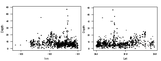
Plots of Depth vs. Latitude and Depth vs. Longitude

Notice the interesting spike in depth of earthquake in both the longitude graph and the latitude graph. With only one of these graphs we would not know whether we had a vertical column of earthquakes going straight down. But with both graphs it becomes obvious that this is precisely what we have.
A portion of our data table shows us precisely where this spike is located. I will use the second to the deepest earthquake for this location as this is the one that seems to be best in line with the rest of the spike.
| Depth | Latitude | Longitude | -------- |
| 56.75 | 37.0725 | -121.393 | Deepest quake |
| 47.51 | 37.1238 | -121.362 | 2nd deepest quake |
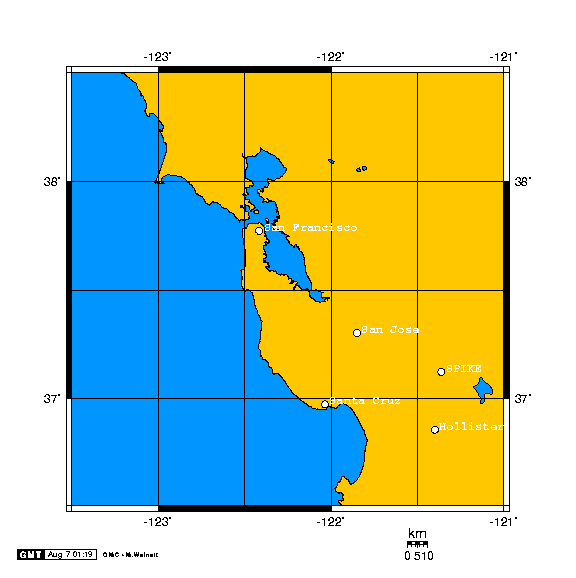
We have a location of for our spike of (37.1238, -121.362). * (latitude, longitude)
The following map will show precisely where this spike of earthquakes is located.
 Courtesy of ON-LINE MAP MAKER, http://www.aquarius.geomar.de/omc/
(Allows making of one’s own map and labeling of specific coordinates)

Again we have a distribution with a skewed tendency toward higher latitudes. We, therefore, see the highest concentration of earthquakes at the low end of our field from 36.5 to around 37.0 degrees latitude.
| Variable | N | Mean | Median | Tr Mean | StDev | SE Mean | Min | Max | Q1 | Q3 |
| Lat | 1356 | 37.170 | 37.052 | 37.141 | 0.504 | 0.014 | 36.500 | 38.490 | 36.768 | 37.509 |
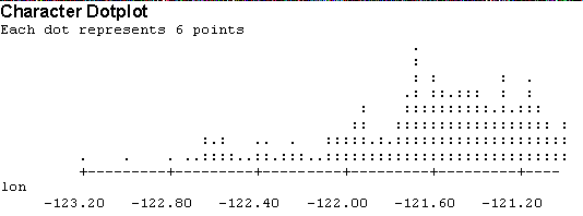
| Lon | 1356 | -121.61 | -121.56 | -121.59 | 0.41 | 0.01 | -123.20 | -121.00 | -121.82 | -121.29 |
The mean latitude of 37.10 compared to the median of 37.052 indicates evidence of skewing toward larger values. 50% of the earthquakes take place in the interquartile range which is [36.768, 37.509]. This is another indication of the concentration in the lower latitudes. The dotplot, however, is the clearest way to see it. The median longitude is -121.56.

Here we have a concentration of earthquakes in the eastern part of our territory from longitude -121.70 to -121.0. Remembering that our concentration of latitude was 36.5 to 37.0, we see that Hollister, CA is in our most concentrated zone. Holister has latitude and longitude of 36.856 and -121.400 respectively.
To see this in a clear manner, I will do a fitted line plot showing how longitude and latitude are related to the number of earthquakes.
The regression equation is y = - 77.6 - 0.944 x
Predictor Coef StDev T P
Constant -77.573 2.657 -29.20 0.000
x -0.94351 0.02184 -43.19 0.000

Our p-value 0f 0.000 is strong evidence that B-1 (beta 1) is not equal to 0. Therefore, we have an association between longitude and latitude as expected from the above dot plots.
S = 0.3272 R-Sq = 57.9% R-Sq(adj) = 57.9%
R-Square tells us that our linear regression model explains 57.9% of the variation in the latitude values.
This is about what I would expect since we have two major faults running through the Bay Area, separated by the San Francisco Bay and accompanied by numerous minor faults scattered throughout the area. It seems logical that this would cause a somewhat wide spread of variation about the regression line.
| Source | DF | SS | MS | F | P |
| Regression | 1 | 199.69 | 199.69 | 1865.54 | 0.000 |
| Error | 1354 | 144.93 | 0.11 | ||
| Total | 1355 | 344.62 | |||
In the above fitted line plot we see a concentration of earthquakes in the lower right hand corner where Hollister is located.
The regression line runs in the same direction as the two major faults through the Bay Area.
Next, we ask the question, “Is the Gutenberg-Richter law working well in the Bay Area?”
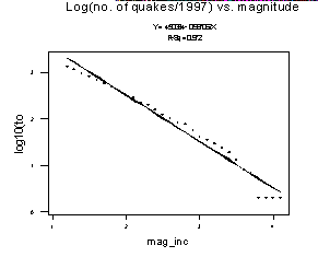
Below is a plot of the log of the no. of quakes greater than or equal to the given magnitude (horizontal axis).
The regression equation is y = 4.50 - 0.997 x

If the Gutenberg-Richter law is working well, we would expect to see a plot close to a straight line with a slope of -1. Our regression equation tells us we have a negative slope of .997. Also, R-Square, the explained variation in log(no. of quakes) = 97.2%.
We have confidence that the Gutenberg-Richter law is working well in the Bay Area. The horizontal dots in the lower right hand corner are due to the fact that there were no earthquakes of 3.8, 3.9,or 4.0. These would surely have been filled in with a larger earthquake sample.
END OF REPORT
Back to Random Number Generators, Statistics, and Probability